Cortical surface-based searchlight decoding

This is a demo for surface-based searchlight decoding, as described in: Chen, Y., Namburi, P., Elliott, L.T., Heinzle, J., Soon, C.S., Chee, M.W.L., and Haynes, J.-D. (2011). Cortical surface-based searchlight decoding. NeuroImage 56, 582–592.

Load Haxby dataset

import pandas as pd
from nilearn import datasets

# We fetch 2nd subject from haxby datasets (which is default)
haxby_dataset = datasets.fetch_haxby()

fmri_filename = haxby_dataset.func[0]
labels = pd.read_csv(haxby_dataset.session_target[0], sep=" ")
y = labels['labels']
session = labels['chunks']

Restrict to faces and houses

from nilearn.image import index_img
condition_mask = y.isin(['face', 'house'])

fmri_img = index_img(fmri_filename, condition_mask)
y, session = y[condition_mask], session[condition_mask]

Surface bold response

from nilearn import datasets, surface
from sklearn import neighbors

# Fetch a coarse surface of the left hemisphere only for speed
fsaverage = datasets.fetch_surf_fsaverage(mesh='fsaverage5')
hemi = 'left'

# Average voxels 5 mm close to the 3d pial surface
radius = 5.
pial_mesh = fsaverage['pial_' + hemi]
X = surface.vol_to_surf(fmri_img, pial_mesh, radius=radius).T

# To define the :term:`BOLD` responses to be included within each searchlight "sphere"
# we define an adjacency matrix based on the inflated surface vertices such
# that nearby surfaces are concatenated within the same searchlight.

infl_mesh = fsaverage['infl_' + hemi]
coords, _ = surface.load_surf_mesh(infl_mesh)
radius = 3.
nn = neighbors.NearestNeighbors(radius=radius)
adjacency = nn.fit(coords).radius_neighbors_graph(coords).tolil()

Searchlight computation

from sklearn.model_selection import KFold
from sklearn.pipeline import make_pipeline
from sklearn.preprocessing import StandardScaler
from sklearn.linear_model import RidgeClassifier
from nilearn.decoding.searchlight import search_light

# Simple linear estimator preceded by a normalization step
estimator = make_pipeline(StandardScaler(),
                          RidgeClassifier(alpha=10.))

# Define cross-validation scheme
cv = KFold(n_splits=3, shuffle=False)

# Cross-validated search light
scores = search_light(X, y, estimator, adjacency, cv=cv, n_jobs=1)

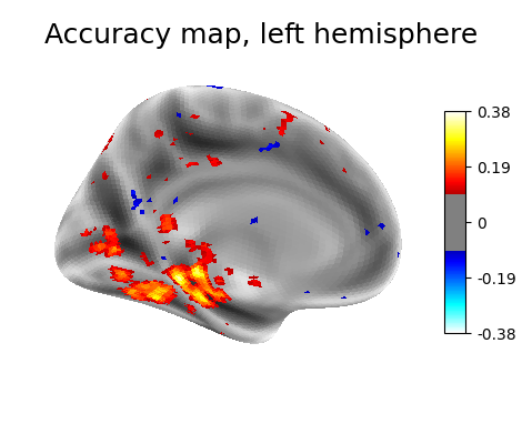
Visualization

from nilearn import plotting
chance = .5
plotting.plot_surf_stat_map(infl_mesh, scores - chance,
                            view='medial', colorbar=True, threshold=0.1,
                            bg_map=fsaverage['sulc_' + hemi],
                            title='Accuracy map, left hemisphere')
plotting.show()

Estimated memory usage: 916 MB