Second-level fMRI model: one sample test

Full step-by-step example of fitting a GLM to perform a second-level analysis (one-sample test) and visualizing the results.

More specifically:

1. A sequence of subject fMRI button press contrasts is downloaded.

2. A mask of the useful brain volume is computed.

3. A one-sample t-test is applied to the brain maps.

We focus on a given contrast of the localizer dataset: the motor response to left versus right button press. Both at the individual and group level, this is expected to elicit activity in the motor cortex (positive in the right hemisphere, negative in the left hemisphere).

Fetch dataset

We download a list of left vs right button press contrasts from a localizer dataset. Note that we fetch individual t-maps that represent the BOLD activity estimate divided by the uncertainty about this estimate.

from nilearn.datasets import fetch_localizer_contrasts

n_subjects = 16
data = fetch_localizer_contrasts(
    ['left vs right button press'],
    n_subjects,
    get_tmaps=True,
    legacy_format=False,
)

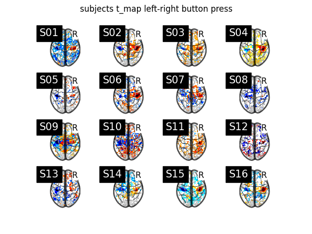
Display subject t_maps

We plot a grid with all the subjects t-maps thresholded at t = 2 for simple visualization purposes. The button press effect is visible among all subjects.

from nilearn import plotting
import matplotlib.pyplot as plt

subjects = data['ext_vars']['participant_id'].tolist()
fig, axes = plt.subplots(nrows=4, ncols=4)
for cidx, tmap in enumerate(data['tmaps']):
    plotting.plot_glass_brain(
        tmap,
        colorbar=False,
        threshold=2.0,
        title=subjects[cidx],
        axes=axes[int(cidx / 4), int(cidx % 4)],
        plot_abs=False,
        display_mode='z',
    )
fig.suptitle('subjects t_map left-right button press')
plt.show()

Estimate second level model

We define the input maps and the design matrix for the second level model and fit it.

import pandas as pd

second_level_input = data['cmaps']
design_matrix = pd.DataFrame(
    [1] * len(second_level_input),
    columns=['intercept'],
)

Model specification and fit.

from nilearn.glm.second_level import SecondLevelModel

second_level_model = SecondLevelModel(smoothing_fwhm=8.0)
second_level_model = second_level_model.fit(
    second_level_input,
    design_matrix=design_matrix,
)

To estimate the contrast is very simple. We can just provide the column name of the design matrix.

z_map = second_level_model.compute_contrast(output_type='z_score')

We threshold the second level contrast at uncorrected p < 0.001 and plot it.

from scipy.stats import norm

p_val = 0.001
p001_unc = norm.isf(p_val)
display = plotting.plot_glass_brain(
    z_map,
    threshold=p001_unc,
    colorbar=True,
    display_mode='z',
    plot_abs=False,
    title='group left-right button press (unc p<0.001)',
)
plotting.show()

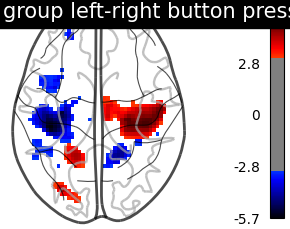
As expected, we find the motor cortex.

Next, we compute the (corrected) p-values with a parametric test to compare them with the results from a nonparametric test.

import numpy as np
from nilearn.image import get_data, math_img

p_val = second_level_model.compute_contrast(output_type='p_value')
n_voxels = np.sum(get_data(second_level_model.masker_.mask_img_))
# Correcting the p-values for multiple testing and taking negative logarithm
neg_log_pval = math_img(
    '-np.log10(np.minimum(1, img * {}))'.format(str(n_voxels)),
    img=p_val,
)

<string>:1: RuntimeWarning: divide by zero encountered in log10

Now, we compute the (corrected) p-values with a permutation test.

Important

In this example, threshold is set to 0.001, which enables cluster-level inference. Performing cluster-level inference will increase the computation time of the permutation procedure. Increasing the number of parallel jobs (n_jobs) can reduce the time cost.

Hint

If you wish to only run voxel-level correction, set threshold to None (the default).

from nilearn.glm.second_level import non_parametric_inference

out_dict = non_parametric_inference(
    second_level_input,
    design_matrix=design_matrix,
    model_intercept=True,
    n_perm=500,  # 500 for the sake of time. Ideally, this should be 10,000.
    two_sided_test=False,
    smoothing_fwhm=8.0,
    n_jobs=1,
    threshold=0.001,
)

/home/alexis/miniconda3/envs/nilearn/lib/python3.10/site-packages/nilearn/mass_univariate/permuted_least_squares.py:960: UserWarning: Data array used to create a new image contains 64-bit ints. This is likely due to creating the array with numpy and passing `int` as the `dtype`. Many tools such as FSL and SPM cannot deal with int64 in Nifti images, so for compatibility the data has been converted to int32.
  image.new_img_like(masker.mask_img_, metric_map),
/home/alexis/miniconda3/envs/nilearn/lib/python3.10/site-packages/nilearn/masking.py:912: UserWarning: Data array used to create a new image contains 64-bit ints. This is likely due to creating the array with numpy and passing `int` as the `dtype`. Many tools such as FSL and SPM cannot deal with int64 in Nifti images, so for compatibility the data has been converted to int32.
  return new_img_like(mask_img, unmasked, affine)

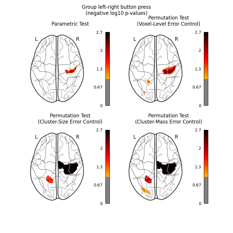
Let us plot the (corrected) negative log p-values for the both tests.

We will use a negative log10 p threshold of 1, which corresponds to p<0.1. This threshold indicates that there is less than 10% probability to make a single false discovery (90% chance that we make no false discovery at all). This threshold is much more conservative than an uncorrected threshold, but is still more liberal than a typical corrected threshold for this kind of analysis, which tends to be ~0.05.

We will also cap the negative log10 p-values at 2.69, because this is the maximum observable value for the nonparametric tests, which were run with only 500 permutations.

threshold = 1  # p < 0.1
vmax = 2.69  # ~= -np.log10(1 / 500)

cut_coords = [0]

IMAGES = [
    neg_log_pval,
    out_dict['logp_max_t'],
    out_dict['logp_max_size'],
    out_dict['logp_max_mass'],
]
TITLES = [
    'Parametric Test',
    'Permutation Test\n(Voxel-Level Error Control)',
    'Permutation Test\n(Cluster-Size Error Control)',
    'Permutation Test\n(Cluster-Mass Error Control)',
]

fig, axes = plt.subplots(figsize=(8, 8), nrows=2, ncols=2)
img_counter = 0
for i_row in range(2):
    for j_col in range(2):
        ax = axes[i_row, j_col]
        plotting.plot_glass_brain(
            IMAGES[img_counter],
            colorbar=True,
            vmax=vmax,
            display_mode='z',
            plot_abs=False,
            cut_coords=cut_coords,
            threshold=threshold,
            figure=fig,
            axes=ax,
        )
        ax.set_title(TITLES[img_counter])
        img_counter += 1

fig.suptitle('Group left-right button press\n(negative log10 p-values)')
plt.show()

/home/alexis/miniconda3/envs/nilearn/lib/python3.10/site-packages/nilearn/_utils/niimg.py:61: UserWarning: Non-finite values detected. These values will be replaced with zeros.
  warn(

The nonparametric test yields many more discoveries and is more powerful than the usual parametric procedure. Even within the nonparametric test, the different correction metrics produce different results. The voxel-level correction is more conservative than the cluster-size or cluster-mass corrections, which are very similar to one another.

Estimated memory usage: 48 MB