Extracting times series to build a functional connectome#
Page summary
A functional connectome is a set of connections representing brain interactions between regions. Here we show how to extract activation time-series to compute functional connectomes.
References
Time-series from a brain parcellation or “MaxProb” atlas#
Brain parcellations#
Regions used to extract the signal can be defined by a “hard”
parcellation. For instance, the nilearn.datasets has functions to
download atlases forming reference parcellation, e.g.,
fetch_atlas_craddock_2012, fetch_atlas_harvard_oxford,
fetch_atlas_yeo_2011.
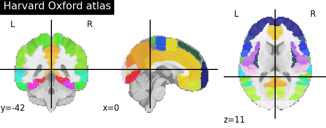
For instance to retrieve the Harvard-Oxford cortical parcellation, sampled at 2mm, and with a threshold of a probability of 0.25:
from nilearn import datasets
dataset = datasets.fetch_atlas_harvard_oxford('cort-maxprob-thr25-2mm')
atlas_filename = dataset.maps
labels = dataset.labels
Plotting can then be done as:
from nilearn import plotting
plotting.plot_roi(atlas_filename)
See also
The dataset downloaders.
Extracting signals on a parcellation#
To extract signal on the parcellation, the easiest option is to use the
NiftiLabelsMasker. As any “maskers” in
nilearn, it is a processing object that is created by specifying all
the important parameters, but not the data:
from nilearn.maskers import NiftiLabelsMasker
masker = NiftiLabelsMasker(labels_img=atlas_filename, standardize=True)
The Nifti data can then be turned to time-series by calling the
NiftiLabelsMasker.fit_transform method, that takes either
filenames or NiftiImage objects:
time_series = masker.fit_transform(frmi_files,
                                   confounds=confounds_dataframe)
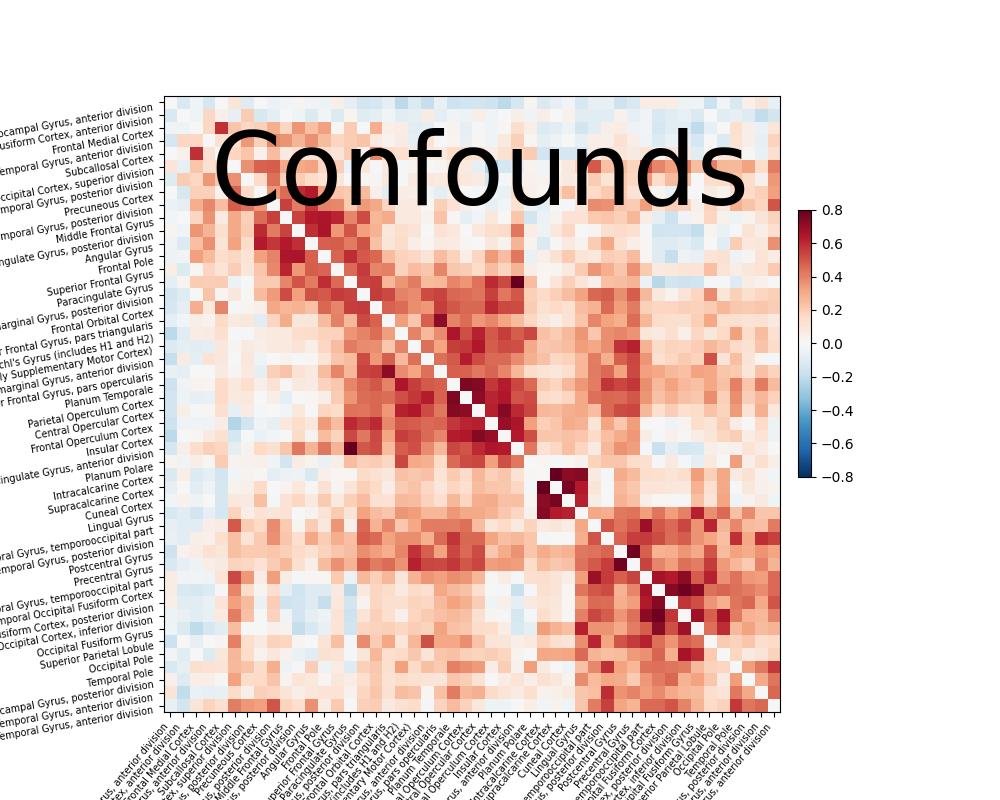
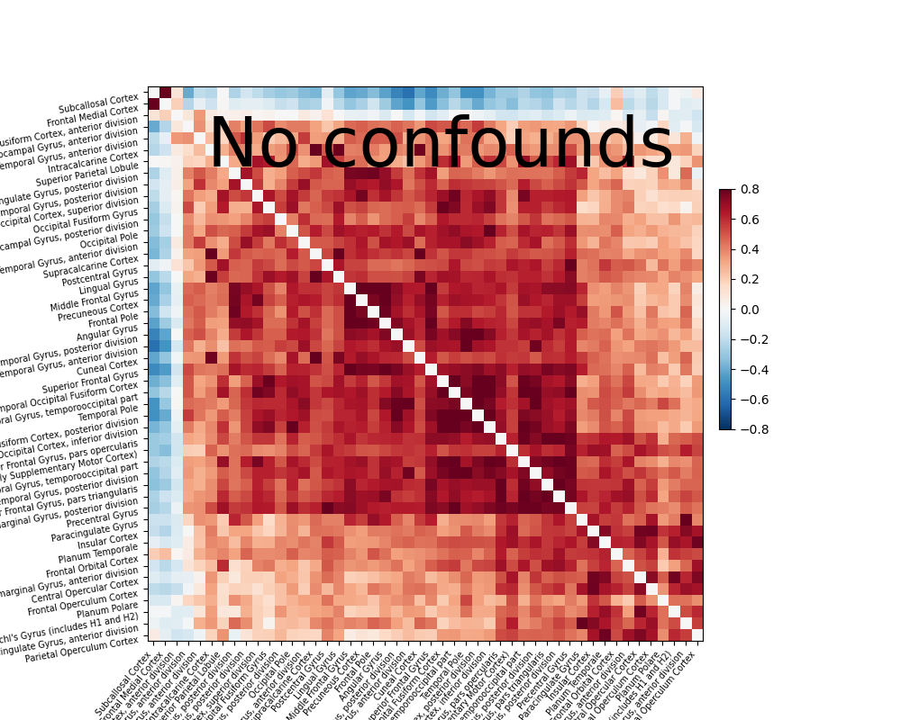
Note that confound signals can be specified in the call. Indeed, to
obtain time series that capture well the functional interactions between
regions, regressing out noise sources is very important
[Varoquaux & Craddock 2013].
For data processed by fMRIPrep,
load_confounds and
load_confounds_strategy can help you
retrieve confound variables.
load_confounds_strategy selects confounds
based on past literature with limited parameters for customisation.
For more freedoms of confounds selection,
load_confounds groups confound variables as
sets of noise components and one can fine tune each of the parameters.
Full example
See the following example for a full file running the analysis: Extracting signals from a brain parcellation.
Exercise: computing the correlation matrix of rest fmri
Try using the information above to compute the correlation matrix of
the first subject of the brain development dataset
downloaded with nilearn.datasets.fetch_development_fmri.
Hints:
Inspect the ‘.keys()’ of the object returned by
nilearn.datasets.fetch_development_fmri.Use
load_confoundsto get a set of confounds of your choice. (Note: CompCor and ICA-AROMA related options are not applicable to the brain development dataset).Use
load_confounds_strategyto get a set of confounds. (Note: onlysimpleandscrubbingare applicable to the brain development dataset).nilearn.connectome.ConnectivityMeasurecan be used to compute a correlation matrix (check the shape of your matrices).matplotlib.pyplot.imshowcan show a correlation matrix.The example above has the solution.
Time-series from a probabilistic atlas#
Probabilistic atlases#
The definition of regions as by a continuous probability map captures
better our imperfect knowledge of boundaries in brain images (notably
because of inter-subject registration errors). One example of such an
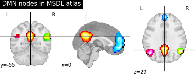
atlas well suited to resting-state or naturalistic-stimuli data analysis is
the MSDL atlas
(nilearn.datasets.fetch_atlas_msdl).
Probabilistic atlases are represented as a set of continuous maps, in a
4D nifti image. Visualization the atlas thus requires to visualize each
of these maps, which requires accessing them with
nilearn.image.index_img (see the corresponding example).
Extracting signals from a probabilistic atlas#
As with extraction of signals on a parcellation, extracting signals from
a probabilistic atlas can be done with a “masker” object: the
NiftiMapsMasker. It is created by
specifying the important parameters, in particular the atlas:
from nilearn.maskers import NiftiMapsMasker
masker = NiftiMapsMasker(maps_img=atlas_filename, standardize=True)
The fit_transform method turns filenames or NiftiImage objects to time series:
time_series = masker.fit_transform(frmi_files, confounds=csv_file)
The procedure is the same as with brain parcellations but using the NiftiMapsMasker, and
the same considerations on using confounds regressors apply.
Full example
A full example of extracting signals on a probabilistic: Extracting signals of a probabilistic atlas of functional regions.
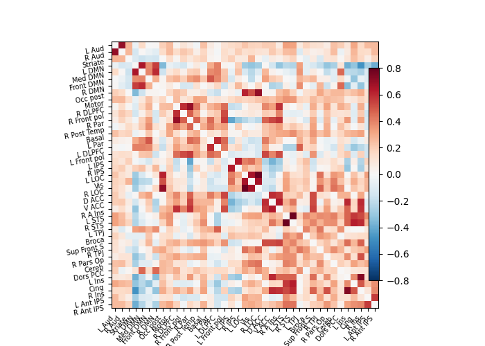
Exercise: correlation matrix of rest fMRI on probabilistic atlas
Try to compute the correlation matrix of the first subject of the
brain development
dataset downloaded with nilearn.datasets.fetch_development_fmri
with the MSDL atlas downloaded via
nilearn.datasets.fetch_atlas_msdl.
Hint: The example above has the solution.
A functional connectome: a graph of interactions#
A square matrix, such as a correlation matrix, can also be seen as a “graph”: a set of “nodes”, connected by “edges”. When these nodes are brain regions, and the edges capture interactions between them, this graph is a “functional connectome”.
We can display it with the nilearn.plotting.plot_connectome
function that take the matrix, and coordinates of the nodes in MNI space.
In the case of the MSDL atlas
(nilearn.datasets.fetch_atlas_msdl), the CSV file readily comes
with MNI coordinates for each region (see for instance example:
Extracting signals of a probabilistic atlas of functional regions).
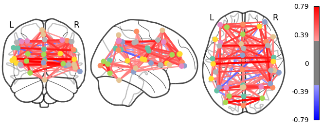
As you can see, the correlation matrix gives a very “full” graph: every node is connected to every other one. This is because it also captures indirect connections. In the next section we will see how to focus on direct connections only.
A functional connectome: extracting coordinates of regions#
For atlases without readily available label coordinates, center coordinates can be computed for each region on hard parcellation or probabilistic atlases.
For hard parcellation atlases (eg.
nilearn.datasets.fetch_atlas_destrieux_2009), use thenilearn.plotting.find_parcellation_cut_coordsfunction. See example: Comparing connectomes on different reference atlasesFor probabilistic atlases (eg.
nilearn.datasets.fetch_atlas_msdl), use thenilearn.plotting.find_probabilistic_atlas_cut_coordsfunction. See example: Group Sparse inverse covariance for multi-subject connectome:>>> from nilearn import plotting >>> atlas_region_coords = plotting.find_probabilistic_atlas_cut_coords(atlas_filename)