BIDS dataset first and second level analysis

Full step-by-step example of fitting a GLM to perform a first and second level analysis in a BIDS dataset and visualizing the results. Details about the BIDS standard can be consulted at http://bids.neuroimaging.io/.

More specifically:

1. Download an fMRI BIDS dataset with two language conditions to contrast.

2. Extract first level model objects automatically from the BIDS dataset.

3. Fit a second level model on the fitted first level models. Notice that in this case the preprocessed bold images were already normalized to the same MNI space.

Fetch example BIDS dataset

We download a simplified BIDS dataset made available for illustrative purposes. It contains only the necessary information to run a statistical analysis using Nilearn. The raw data subject folders only contain bold.json and events.tsv files, while the derivatives folder includes the preprocessed files preproc.nii and the confounds.tsv files.

from nilearn.datasets import fetch_language_localizer_demo_dataset
data_dir, _ = fetch_language_localizer_demo_dataset()

Dataset created in /home/alexis/nilearn_data/fMRI-language-localizer-demo-dataset

Downloading data from https://osf.io/3dj2a/download ...

Downloaded 17768448 of 749503182 bytes (2.4%,   41.6s remaining)
Downloaded 57712640 of 749503182 bytes (7.7%,   24.1s remaining)
Downloaded 99221504 of 749503182 bytes (13.2%,   19.7s remaining)
Downloaded 143597568 of 749503182 bytes (19.2%,   16.9s remaining)
Downloaded 188817408 of 749503182 bytes (25.2%,   14.9s remaining)
Downloaded 226942976 of 749503182 bytes (30.3%,   13.8s remaining)
Downloaded 270843904 of 749503182 bytes (36.1%,   12.4s remaining)
Downloaded 317079552 of 749503182 bytes (42.3%,   10.9s remaining)
Downloaded 358080512 of 749503182 bytes (47.8%,    9.9s remaining)
Downloaded 404078592 of 749503182 bytes (53.9%,    8.6s remaining)
Downloaded 440090624 of 749503182 bytes (58.7%,    7.7s remaining)
Downloaded 479420416 of 749503182 bytes (64.0%,    6.8s remaining)
Downloaded 521510912 of 749503182 bytes (69.6%,    5.7s remaining)
Downloaded 565444608 of 749503182 bytes (75.4%,    4.6s remaining)
Downloaded 609492992 of 749503182 bytes (81.3%,    3.4s remaining)
Downloaded 646275072 of 749503182 bytes (86.2%,    2.6s remaining)
Downloaded 683892736 of 749503182 bytes (91.2%,    1.6s remaining)
Downloaded 728293376 of 749503182 bytes (97.2%,    0.5s remaining) ...done. (20 seconds, 0 min)
Extracting data from /home/alexis/nilearn_data/fMRI-language-localizer-demo-dataset/fMRI-language-localizer-demo-dataset.zip..... done.

Here is the location of the dataset on disk.

print(data_dir)

/home/alexis/nilearn_data/fMRI-language-localizer-demo-dataset

Obtain automatically FirstLevelModel objects and fit arguments

From the dataset directory we automatically obtain the FirstLevelModel objects with their subject_id filled from the BIDS dataset. Moreover, we obtain for each model a dictionary with run_imgs, events and confounder regressors since in this case a confounds.tsv file is available in the BIDS dataset. To get the first level models we only have to specify the dataset directory and the task_label as specified in the file names.

from nilearn.glm.first_level import first_level_from_bids
task_label = 'languagelocalizer'
models, models_run_imgs, models_events, models_confounds = \
    first_level_from_bids(
        data_dir, task_label,
        img_filters=[('desc', 'preproc')])

/home/alexis/miniconda3/envs/nilearn/lib/python3.10/site-packages/nilearn/glm/first_level/first_level.py:901: UserWarning:

SliceTimingRef not found in file /home/alexis/nilearn_data/fMRI-language-localizer-demo-dataset/derivatives/sub-01/func/sub-01_task-languagelocalizer_desc-preproc_bold.json. It will be assumed that the slice timing reference is 0.0 percent of the repetition time. If it is not the case it will need to be set manually in the generated list of models

Quick sanity check on fit arguments

Additional checks or information extraction from pre-processed data can be made here.

We just expect one run_img per subject.

import os
print([os.path.basename(run) for run in models_run_imgs[0]])

['sub-01_task-languagelocalizer_desc-preproc_bold.nii.gz']

The only confounds stored are regressors obtained from motion correction. As we can verify from the column headers of the confounds table corresponding to the only run_img present.

print(models_confounds[0][0].columns)

Index(['RotX', 'RotY', 'RotZ', 'X', 'Y', 'Z'], dtype='object')

During this acquisition the subject read blocks of sentences and consonant strings. So these are our only two conditions in events. We verify there are 12 blocks for each condition.

print(models_events[0][0]['trial_type'].value_counts())

language    12
string      12
Name: trial_type, dtype: int64

First level model estimation

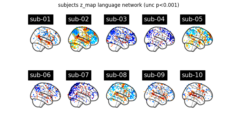
Now we simply fit each first level model and plot for each subject the contrast that reveals the language network (language - string). Notice that we can define a contrast using the names of the conditions specified in the events dataframe. Sum, subtraction and scalar multiplication are allowed.

Set the threshold as the z-variate with an uncorrected p-value of 0.001.

from scipy.stats import norm
p001_unc = norm.isf(0.001)

Prepare figure for concurrent plot of individual maps.

from nilearn import plotting
import matplotlib.pyplot as plt

fig, axes = plt.subplots(nrows=2, ncols=5, figsize=(8, 4.5))
model_and_args = zip(models, models_run_imgs, models_events, models_confounds)
for midx, (model, imgs, events, confounds) in enumerate(model_and_args):
    # fit the GLM
    model.fit(imgs, events, confounds)
    # compute the contrast of interest
    zmap = model.compute_contrast('language-string')
    plotting.plot_glass_brain(zmap, colorbar=False, threshold=p001_unc,
                              title=('sub-' + model.subject_label),
                              axes=axes[int(midx / 5), int(midx % 5)],
                              plot_abs=False, display_mode='x')
fig.suptitle('subjects z_map language network (unc p<0.001)')
plotting.show()

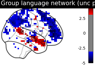
Second level model estimation

We just have to provide the list of fitted FirstLevelModel objects to the SecondLevelModel object for estimation. We can do this because all subjects share a similar design matrix (same variables reflected in column names).

from nilearn.glm.second_level import SecondLevelModel
second_level_input = models

Note that we apply a smoothing of 8mm.

second_level_model = SecondLevelModel(smoothing_fwhm=8.0)
second_level_model = second_level_model.fit(second_level_input)

Computing contrasts at the second level is as simple as at the first level. Since we are not providing confounders we are performing a one-sample test at the second level with the images determined by the specified first level contrast.

zmap = second_level_model.compute_contrast(
    first_level_contrast='language-string')

The group level contrast reveals a left lateralized fronto-temporal language network.

plotting.plot_glass_brain(zmap, colorbar=True, threshold=p001_unc,
                          title='Group language network (unc p<0.001)',
                          plot_abs=False, display_mode='x')
plotting.show()

Estimated memory usage: 188 MB