Note
This page is a reference documentation. It only explains the function signature, and not how to use it. Please refer to the user guide for the big picture.
nilearn.plotting.view_img#
- nilearn.plotting.view_img(stat_map_img, bg_img='MNI152', cut_coords=None, colorbar=True, title=None, threshold=1e-06, annotate=True, draw_cross=True, black_bg='auto', cmap=<matplotlib.colors.LinearSegmentedColormap object>, symmetric_cmap=True, dim='auto', vmax=None, vmin=None, resampling_interpolation='continuous', opacity=1, **kwargs)[source]#
Interactive html viewer of a statistical map, with optional background.
- Parameters
- stat_map_imgNiimg-like object
See http://nilearn.github.io/manipulating_images/input_output.html The statistical map image. Can be either a 3D volume or a 4D volume with exactly one time point.
- bg_imgNiimg-like object, optional
See input_output. The background image to plot on top of. If nothing is specified, the MNI152 template will be used. To turn off background image, just pass “bg_img=False”. Default=’MNI152’.
- cut_coordsNone, or a tuple of floats
The MNI coordinates of the point where the cut is performed as a 3-tuple: (x, y, z). If None is given, the cuts are calculated automatically.
- colorbarboolean, optional
If True, display a colorbar on top of the plots. Default=True.
- title
str, or None, optional The title displayed on the figure. Default=None.
- thresholdstring, number or None, optional
If None is given, the image is not thresholded. If a string of the form “90%” is given, use the 90-th percentile of the absolute value in the image. If a number is given, it is used to threshold the image: values below the threshold (in absolute value) are plotted as transparent. If auto is given, the threshold is determined automatically. Default=1e-6.
- annotateboolean, optional
If annotate is True, current cuts are added to the viewer. Default=True.
- draw_cross
bool, optional If
draw_crossisTrue, a cross is drawn on the plot to indicate the cut position. Default=True.- black_bgboolean or ‘auto’, optional
If True, the background of the image is set to be black. Otherwise, a white background is used. If set to auto, an educated guess is made to find if the background is white or black. Default=’auto’.
- cmap
matplotlib.colors.Colormap, orstr, optional The colormap to use. Either a string which is a name of a matplotlib colormap, or a matplotlib colormap object. Default=`plt.cm.cold_hot`.
- symmetric_cmapbool, optional
True: make colormap symmetric (ranging from -vmax to vmax). False: the colormap will go from the minimum of the volume to vmax. Set it to False if you are plotting a positive volume, e.g. an atlas or an anatomical image. Default=True.
- dim
float, or ‘auto’, optional Dimming factor applied to background image. By default, automatic heuristics are applied based upon the background image intensity. Accepted float values, where a typical span is between -2 and 2 (-2 = increase contrast; 2 = decrease contrast), but larger values can be used for a more pronounced effect. 0 means no dimming. Default=’auto’.
- vmaxfloat, or None, optional
max value for mapping colors. If vmax is None and symmetric_cmap is True, vmax is the max absolute value of the volume. If vmax is None and symmetric_cmap is False, vmax is the max value of the volume.
- vminfloat, or None, optional
min value for mapping colors. If symmetric_cmap is True, vmin is always equal to -vmax and cannot be chosen. If symmetric_cmap is False, vmin defaults to the min of the image, or 0 when a threshold is used.
- resampling_interpolation
str, optional Interpolation to use when resampling the image to the destination space. Can be:
“continuous”: use 3rd-order spline interpolation
“nearest”: use nearest-neighbor mapping.
Note
“nearest” is faster but can be noisier in some cases.
Default=’continuous’.
- opacityfloat in [0,1], optional
The level of opacity of the overlay (0: transparent, 1: opaque). Default=1.
- Returns
- html_viewthe html viewer object.
It can be saved as an html page html_view.save_as_html(‘test.html’), or opened in a browser html_view.open_in_browser(). If the output is not requested and the current environment is a Jupyter notebook, the viewer will be inserted in the notebook.
See also
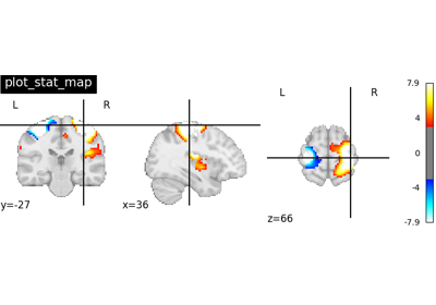
nilearn.plotting.plot_stat_mapstatic plot of brain volume, on a single or multiple planes.
nilearn.plotting.view_connectomeinteractive 3d view of a connectome.
nilearn.plotting.view_markersinteractive plot of colored markers.
nilearn.plotting.view_surf,nilearn.plotting.view_img_on_surfinteractive view of statistical maps or surface atlases on the cortical surface.
Examples using nilearn.plotting.view_img#
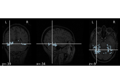
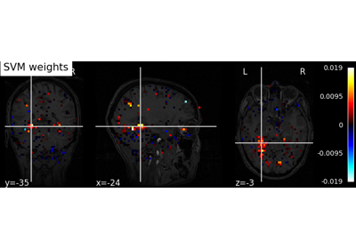
Decoding with ANOVA + SVM: face vs house in the Haxby dataset