Note

This page is a reference documentation. It only explains the class signature, and not how to use it. Please refer to the user guide for the big picture.

nilearn.plotting.displays.XProjector

class nilearn.plotting.displays.XProjector(cut_coords, axes=None, black_bg=False, brain_color=(0.5, 0.5, 0.5), **kwargs)

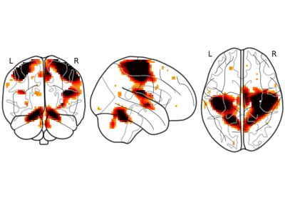
The XProjector class enables sagittal visualization through 2D projections with plot_glass_brain. This visualization mode can be activated by setting display_mode='x':

from nilearn.datasets import load_mni152_template
from nilearn.plotting import plot_glass_brain
img = load_mni152_template()
# display is an instance of the XProjector class
display = plot_glass_brain(img, display_mode='x')

See also

nilearn.plotting.displays.YProjector

Coronal view

nilearn.plotting.displays.ZProjector

Axial view

Attributes

axesdict of GlassBrainAxes

The axes used for plotting.

frame_axesAxes

The axes framing the whole set of views.

__init__(cut_coords, axes=None, black_bg=False, brain_color=(0.5, 0.5, 0.5), **kwargs)

add_contours(img, threshold=1e-06, filled=False, **kwargs)

Contour a 3D map in all the views.

Parameters

imgNiimg-like object

See input-output. Provides image to plot.

thresholdint or float or None, optional

Threshold to apply:

• If None is given, the maps are not thresholded.

• If a number is given, it is used to threshold the maps, values below the threshold (in absolute value) are plotted as transparent.

Default=1e-6.

filledbool, optional

If filled=True, contours are displayed with color fillings. Default=False.

kwargsdict

Extra keyword arguments are passed to function contour, or function contourf. Useful, arguments are typical “levels”, which is a list of values to use for plotting a contour or contour fillings (if filled=True), and “colors”, which is one color or a list of colors for these contours.

Notes

If colors are not specified, default coloring choices (from matplotlib) for contours and contour_fillings can be different.

add_edges(img, color='r')

Plot the edges of a 3D map in all the views.

Parameters

imgNiimg-like object

See input-output. The 3D map to be plotted. If it is a masked array, only the non-masked part will be plotted.

colormatplotlib color: str or (r, g, b) value

The color used to display the edge map. Default=’r’.

add_graph(adjacency_matrix, node_coords, node_color='auto', node_size=50, edge_cmap=<matplotlib.colors.LinearSegmentedColormap object>, edge_vmin=None, edge_vmax=None, edge_threshold=None, edge_kwargs=None, node_kwargs=None, colorbar=False)

Plot undirected graph on each of the axes.

Parameters

adjacency_matrixnumpy.ndarray of shape (n, n)

Represents the edges strengths of the graph. The matrix can be symmetric which will result in an undirected graph, or not symmetric which will result in a directed graph.

node_coordsnumpy.ndarray of shape (n, 3)

3D coordinates of the graph nodes in world space.

node_colorcolor or sequence of colors, optional

Color(s) of the nodes. Default=’auto’.

node_sizescalar or array_like, optional

Size(s) of the nodes in points^2. Default=50.

edge_cmapColormap, optional

Colormap used for representing the strength of the edges. Default=cm.bwr.

edge_vmin, edge_vmaxfloat, optional

• If not None, either or both of these values will be used to as the minimum and maximum values to color edges.

• If None are supplied, the maximum absolute value within the given threshold will be used as minimum (multiplied by -1) and maximum coloring levels.

edge_thresholdstr or int or float, optional

• If it is a number only the edges with a value greater than edge_threshold will be shown.

• If it is a string it must finish with a percent sign, e.g. “25.3%”, and only the edges with a abs(value) above the given percentile will be shown.

edge_kwargsdict, optional

Will be passed as kwargs for each edge Line2D.

node_kwargsdict

Will be passed as kwargs to the function scatter which plots all the nodes at one.

add_markers(marker_coords, marker_color='r', marker_size=30, **kwargs)

Add markers to the plot.

Parameters

marker_coordsndarray of shape (n_markers, 3)

Coordinates of the markers to plot. For each slice, only markers that are 2 millimeters away from the slice are plotted.

marker_colorpyplot compatible color or list of shape (n_markers,), optional

List of colors for each marker that can be string or matplotlib colors. Default=’r’.

marker_sizefloat or list of float of shape (n_markers,), optional

Size in pixel for each marker. Default=30.

add_overlay(img, threshold=1e-06, colorbar=False, cbar_tick_format='%.2g', cbar_vmin=None, cbar_vmax=None, **kwargs)

Plot a 3D map in all the views.

Parameters

imgNiimg-like object

See input-output. If it is a masked array, only the non-masked part will be plotted.

thresholdint or float or None, optional

Threshold to apply:

• If None is given, the maps are not thresholded.

• If a number is given, it is used to threshold the maps: values below the threshold (in absolute value) are plotted as transparent.

Default=1e-6.

cbar_tick_format: str, optional

Controls how to format the tick labels of the colorbar. Ex: use “%i” to display as integers. Default is ‘%.2g’ for scientific notation.

colorbarbool, optional

If True, display a colorbar on the right of the plots. Default=False.

kwargsdict

Extra keyword arguments are passed to function imshow.

cbar_vminfloat, optional

Minimal value for the colorbar. If None, the minimal value is computed based on the data.

cbar_vmaxfloat, optional

Maximal value for the colorbar. If None, the maximal value is computed based on the data.

annotate(left_right=True, positions=True, scalebar=False, size=12, scale_size=5.0, scale_units='cm', scale_loc=4, decimals=0, **kwargs)

Add annotations to the plot.

Parameters

left_rightbool, optional

If True, annotations indicating which side is left and which side is right are drawn. Default=True.

positionsbool, optional

If True, annotations indicating the positions of the cuts are drawn. Default=True.

scalebarbool, optional

If True, cuts are annotated with a reference scale bar. For finer control of the scale bar, please check out the draw_scale_bar method on the axes in “axes” attribute of this object. Default=False.

sizeint, optional

The size of the text used. Default=12.

scale_sizeint or float, optional

The length of the scalebar, in units of scale_units. Default=5.0.

scale_units{‘cm’, ‘mm’}, optional

The units for the scalebar. Default=’cm’.

scale_locint, optional

The positioning for the scalebar. Default=4. Valid location codes are:

• 1: “upper right”

• 2: “upper left”

• 3: “lower left”

• 4: “lower right”

• 5: “right”

• 6: “center left”

• 7: “center right”

• 8: “lower center”

• 9: “upper center”

• 10: “center”

decimalsint, optional

Number of decimal places on slice position annotation. If zero, the slice position is integer without decimal point. Default=0.

kwargsdict

Extra keyword arguments are passed to matplotlib’s text function.

property black_bg

property brain_color

close()

Close the figure. This is necessary to avoid leaking memory.

draw_cross(cut_coords=None, **kwargs)

Draw a crossbar on the plot to show where the cut is performed.

Parameters

cut_coords3-tuple of float, optional

The position of the cross to draw. If None is passed, the OrthoSlicer’s cut coordinates are used.

kwargsdict

Extra keyword arguments are passed to function axhline.

classmethod find_cut_coords(img=None, threshold=None, cut_coords=None)

Instantiate the slicer and find cut coordinates.

Parameters

%(img)s

thresholdint or float or None, optional

Threshold to apply:

• If None is given, the maps are not thresholded.

• If a number is given, it is used to threshold the maps, values below the threshold (in absolute value) are plotted as transparent.

Default=None.

cut_coords3 tuple of int

The cut position, in world space.

classmethod init_with_figure(img, threshold=None, cut_coords=None, figure=None, axes=None, black_bg=False, leave_space=False, colorbar=False, brain_color=(0.5, 0.5, 0.5), **kwargs)

Initialize the slicer with an image.

Parameters

imgNiimg-like object

See input-output.

cut_coords3 tuple of int

The cut position, in world space.

axesmatplotlib.axes.Axes, optional

The axes that will be subdivided in 3.

black_bgbool, optional

If True, the background of the figure will be put to black. If you wish to save figures with a black background, you will need to pass facecolor='k', edgecolor='k' to matplotlib.pyplot.savefig. Default=False.

brain_colortuple, optional

The brain color to use as the background color (e.g., for transparent colorbars). Default=(0.5, 0.5, 0.5).

savefig(filename, dpi=None)

Save the figure to a file.

Parameters

filenamestr

The file name to save to. Its extension determines the file type, typically ‘.png’, ‘.svg’ or ‘.pdf’.

dpiNone or scalar, optional

The resolution in dots per inch. Default=None.

title(text, x=0.01, y=0.99, size=15, color=None, bgcolor=None, alpha=1, **kwargs)

Write a title to the view.

Parameters

textstr

The text of the title.

xfloat, optional

The horizontal position of the title on the frame in fraction of the frame width. Default=0.01.

yfloat, optional

The vertical position of the title on the frame in fraction of the frame height. Default=0.99.

sizeint, optional

The size of the title text. Default=15.

colormatplotlib color specifier, optional

The color of the font of the title.

bgcolormatplotlib color specifier, optional

The color of the background of the title.

alphafloat, optional

The alpha value for the background. Default=1.

kwargs

Extra keyword arguments are passed to matplotlib’s text function.

Examples using nilearn.plotting.displays.XProjector

Glass brain plotting in nilearn (all options)

Glass brain plotting in nilearn (all options)