Introduction#
What is nilearn: MVPA, decoding, predictive models, functional connectivity#
Why use nilearn?
Nilearn makes it easy to use many advanced machine learning, pattern recognition and multivariate statistical techniques on neuroimaging data for applications such as MVPA (Mutli-Voxel Pattern Analysis), decoding, predictive modelling, functional connectivity, brain parcellations, connectomes.
Nilearn can readily be used on task fMRI, resting-state, or VBM data.
For a machine-learning expert, the value of nilearn can be seen as domain-specific feature engineering construction, that is, shaping neuroimaging data into a feature matrix well suited to statistical learning, or vice versa.
Why is machine learning relevant to NeuroImaging? A few examples!#
- Diagnosis and prognosis
Predicting a clinical score or even treatment response from brain imaging with supervised learning e.g. [Mourao-Miranda 2012]
- Measuring generalization scores
Information mapping: using the prediction accuracy of a classifier to characterize relationships between brain images and stimuli. (e.g. searchlight) [Kriegeskorte 2005]
Transfer learning: measuring how much an estimator trained on one specific psychological process/task can predict the neural activity underlying another specific psychological process/task (e.g. discriminating left from right eye movements also discriminates additions from subtractions [Knops 2009])
- High-dimensional multivariate statistics
From a statistical point of view, machine learning implements statistical estimation of models with a large number of parameters. Tricks pulled in machine learning (e.g. regularization) can make this estimation possible despite the usually small number of observations in the neuroimaging domain [Varoquaux 2012]. This usage of machine learning requires some understanding of the models.
- Data mining / exploration
Data-driven exploration of brain images. This includes the extraction of the major brain networks from resting-state data (“resting-state networks”) or movie-watching data as well as the discovery of connectionally coherent functional modules (“connectivity-based parcellation”). For example, Extracting functional brain networks: ICA and related or Clustering to parcellate the brain in regions with clustering.
Installing nilearn#
1. Setup a virtual environment
We recommend that you install nilearn
in a virtual Python environment, either managed
with the standard library venv
or with conda (see miniconda for instance).
Either way, create and activate a new python environment.
With venv:
python3 -m venv /<path_to_new_env>
source /<path_to_new_env>/bin/activate
Windows users should change the last line to \<path_to_new_env>\Scripts\activate.bat
in order to activate their virtual environment.
With conda:
conda create -n nilearn python=3.9
conda activate nilearn
2. Install nilearn with pip
Execute the following command in the command prompt / terminal in the proper python environment:
python -m pip install -U nilearn
3. Check installation
Try importing nilearn in a python / iPython session:
import nilearn
If no error is raised, you have installed nilearn correctly.
In order to access the development version of nilearn, simply clone and go to the repo:
git clone https://github.com/nilearn/nilearn.git
cd nilearn
Install the package in the proper conda environment with
python -m pip install -r requirements-dev.txt
python -m pip install -e .
To check your install, try importing nilearn in a python session:
import nilearn
If no error is raised, you have installed nilearn correctly.
Python for NeuroImaging, a quick start#
If you don’t know Python, Don’t panic. Python is easy. It is important to realize that most things you will do in nilearn require only a few or a few dozen lines of Python code. Here, we give the basics to help you get started. For a very quick start into the programming language, you can learn it online. For a full-blown introduction to using Python for science, see the scipy lecture notes.
We will be using Jupyter for notebooks, or IPython, which provides an interactive scientific environment that facilitates many everyday data-manipulation steps (e.g. interactive debugging, easy visualization). You can choose notebooks or terminal:
- Notebooks
Start the Jupyter notebook either with the application menu, or by typing:
jupyter notebook
- Terminal
Start iPython by typing:
ipython --matplotlib
Note
The
--matplotlibflag, which configures matplotlib for interactive use inside IPython.
These will give you a prompt in which you can execute commands:
In [1]: 1 + 2 * 3
Out[1]: 7
>>> Prompt
Below we’ll be using >>> to indicate input lines. If you wish to copy and paste these input lines directly, click on the >>> located at the top right of the code block to toggle these prompt signs
Your first steps with nilearn#
First things first, nilearn does not have a graphical user interface. But you will soon realize that you don’t really need one. It is typically used interactively in IPython or in an automated way by Python code. Most importantly, nilearn functions that process neuroimaging data accept either a filename (i.e., a string variable) or a NiftiImage object. We call the latter “niimg-like”.
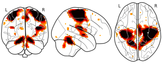
Suppose for instance that you have a Tmap image saved in the Nifti file “t_map000.nii” in the directory “/home/user”. To visualize that image, you will first have to import the plotting functionality by:
>>> from nilearn import plotting
Then you can call the function that creates a “glass brain” by giving it the file name:
>>> plotting.plot_glass_brain("/home/user/t_map000.nii")
Note
There are many other plotting functions. Take your time to have a look at the different options.
For simple functions/operations on images, many functions exist, such as in
the nilearn.image module for image manipulation, e.g.
image.smooth_img for smoothing:
>>> from nilearn import image
>>> smoothed_img = image.smooth_img("/home/user/t_map000.nii", fwhm=5)
The returned value smoothed_img is a NiftiImage object. It can either be passed to other nilearn functions operating on niimgs (neuroimaging images) or saved to disk with:
>>> smoothed_img.to_filename("/home/user/t_map000_smoothed.nii")
Finally, nilearn deals with Nifti images that come in two flavors: 3D
images, which represent a brain volume, and 4D images, which represent a
series of brain volumes. To extract the n-th 3D image from a 4D image, you can
use the image.index_img function (keep in mind that array indexing
always starts at 0 in the Python language):
>>> first_volume = image.index_img("/home/user/fmri_volumes.nii", 0)
To loop over each individual volume of a 4D image, use image.iter_img:
>>> for volume in image.iter_img("/home/user/fmri_volumes.nii"):
...     smoothed_img = image.smooth_img(volume, fwhm=5)
Exercise: varying the amount of smoothing
Want to sharpen your skills with nilearn?
Compute the mean EPI for first subject of the brain development
dataset downloaded with nilearn.datasets.fetch_development_fmri and
smooth it with an FWHM varying from 0mm to 20mm in increments of 5mm
Hints:
Inspect the ‘.keys()’ of the object returned by
nilearn.datasets.fetch_development_fmriLook at the “reference” section of the documentation: there is a function to compute the mean of a 4D image
To perform a for loop in Python, you can use the “range” function
The solution can be found here
Tutorials to learn the basics
The two following tutorials may be useful to get familiar with data representation in nilearn:
More tutorials can be found here
Now, if you want out-of-the-box methods to process neuroimaging data, jump directly to the section you need:
Scientific computing with Python#
In case you plan to become a casual nilearn user, note that you will not need to deal with number and array manipulation directly in Python. However, if you plan to go beyond that, here are a few pointers.
Basic numerics#
- Numerical arrays
The numerical data (e.g. matrices) are stored in numpy arrays:
>>> import numpy as np
>>> t = np.linspace(1, 10, 2000)  # 2000 points between 1 and 10
>>> t
array([  1.        ,   1.00450225,   1.0090045 , ...,   9.9909955 ,
         9.99549775,  10.        ])
>>> t / 2
array([ 0.5       ,  0.50225113,  0.50450225, ...,  4.99549775,
        4.99774887,  5.        ])
>>> np.cos(t) # Operations on arrays are defined in the numpy module
array([ 0.54030231,  0.53650833,  0.53270348, ..., -0.84393609,
       -0.84151234, -0.83907153])
>>> t[:3] # In Python indexing is done with [] and starts at zero
array([ 1.        ,  1.00450225,  1.0090045 ])
Warning
the default integer type used by Numpy is (signed) 64-bit. Several popular neuroimaging tools do not handle int64 Nifti images, so if you build Nifti images directly from Numpy arrays it is recommended to specify a smaller integer type, for example:
np.array([1, 2000, 7], dtype="int32")
- Plotting and figures
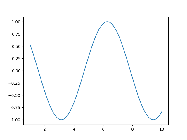
>>> import matplotlib.pyplot as plt
>>> plt.plot(t, np.cos(t))
[<matplotlib.lines.Line2D object at ...>]
- Image processing
>>> from scipy.ndimage import gaussian_filter
>>> t_smooth = gaussian_filter(t, sigma=2)
- Signal processing
>>> from scipy import signal
>>> t_detrended = signal.detrend(t)
- Much more
Simple statistics:
>>> from scipy import stats
Linear algebra:
>>> from scipy import linalg
Scikit-learn: machine learning in Python#
What is scikit-learn?
Scikit-learn is a Python library for machine learning. Its strong points are:
Easy to use and well documented
Computationally efficient
Provides a wide variety of standard machine learning methods for non-experts
The core concept in scikit-learn is the estimator object, for instance an SVC (support vector classifier). It is first created with the relevant parameters:
>>> import sklearn; sklearn.set_config(print_changed_only=False)
>>> from sklearn.svm import SVC
>>> svc = SVC(kernel='linear', C=1.)
These parameters are detailed in the documentation of the object: in IPython or Jupyter you can do:
In [3]: SVC?
...
Parameters
----------
C : float or None, optional (default=None)
    Penalty parameter C of the error term. If None then C is set
    to n_samples.

kernel : string, optional (default='rbf')
    Specifies the kernel type to be used in the algorithm.
    It must be one of 'linear', 'poly', 'rbf', 'sigmoid', 'precomputed'.
    If none is given, 'rbf' will be used.
...
Once the object is created, you can fit it on data. For instance, here we use a hand-written digits dataset, which comes with scikit-learn:
>>> from sklearn import datasets
>>> digits = datasets.load_digits()
>>> data = digits.data
>>> labels = digits.target
Let’s use all but the last 10 samples to train the SVC:
>>> svc.fit(data[:-10], labels[:-10])
SVC(C=1.0, ...)
and try predicting the labels on the left-out data:
>>> svc.predict(data[-10:])
array([5, 4, 8, 8, 4, 9, 0, 8, 9, 8])
>>> labels[-10:]    # The actual labels
array([5, 4, 8, 8, 4, 9, 0, 8, 9, 8])
To find out more, try the scikit-learn tutorials.
Finding help#
- Reference material
A quick and gentle introduction to scientific computing with Python can be found in the scipy lecture notes.
The documentation of scikit-learn explains each method with tips on practical use and examples: http://scikit-learn.org/. While not specific to neuroimaging, it is often a recommended read. Be careful to consult the documentation of the scikit-learn version that you are using.
- Mailing lists and forums
Don’t hesitate to ask questions about nilearn on neurostars.
You can find help with neuroimaging in Python (file I/O, neuroimaging-specific questions) via the nipy user group: https://groups.google.com/forum/?fromgroups#!forum/nipy-user
For machine-learning and scikit-learn questions, expertise can be found on the scikit-learn mailing list: https://mail.python.org/mailman/listinfo/scikit-learn