Clustering to parcellate the brain in regions#
This page discusses how clustering can be used to parcellate the brain into homogeneous regions from functional imaging data.
Reference
A big-picture reference on the use of clustering for brain parcellations.
Thirion, et al. “Which fMRI clustering gives good brain parcellations?.” Frontiers in neuroscience 8.167 (2014): 13.
Data loading: movie-watching data#
Clustering is commonly applied to resting-state data, but any brain
functional data will give rise of a functional parcellation, capturing
intrinsic brain architecture in the case of resting-state data.
In the examples, we use naturalistic stimuli-based movie watching
brain development data downloaded with the function
fetch_development_fmri (see Inputing data: file names or image objects).
Applying clustering#
Which clustering to use
The question of which clustering method to use is in itself subject to debate. There are many clustering methods; their computational cost will vary, as well as their results. A well-cited empirical comparison paper, Thirion et al. 2014 suggests that:
For a large number of clusters, it is preferable to use Ward agglomerative clustering with spatial constraints
For a small number of clusters, it is preferable to use Kmeans clustering after spatially-smoothing the data.
Both algorithms are provided by this object
nilearn.regions.Parcellations as well as two algorithms
tailored to more specific usecases:
nilearn.regions.ReNAis a quicker alternative to Ward with a small loss of precision, it is ideal to downsize the number of voxels by 10 quickly.Hierarchical KMeans is useful to obtain a small number of clusters after spatial smoothing, that will be better balanced than with Kmeans.
All these algorithms are showcased in a full code example : here. Below, we focus on explaining the principle of Ward.
Compute a connectivity matrix Before applying Ward’s method, we compute a spatial neighborhood matrix, aka connectivity matrix. This is useful to constrain clusters to form contiguous parcels (see the scikit-learn documentation)
This is done from the mask computed by the masker: a niimg from which we extract a numpy array and then the connectivity matrix.
Ward clustering principle Ward’s algorithm is a hierarchical clustering algorithm: it recursively merges voxels, then clusters that have similar signal (parameters, measurements or time courses).
Caching In practice the implementation of Ward clustering first computes a tree of possible merges, and then, given a requested number of clusters, breaks apart the tree at the right level.
As the tree is independent of the number of clusters, we can rely on caching to speed things up when varying the number of clusters. In Wards clustering, the memory parameter is used to cache the computed component tree. You can give it either a joblib.Memory instance or the name of a directory used for caching.
Note
The Ward clustering computing 1000 parcels runs typically in about 10 seconds. Admittedly, this is very fast.
Note
The steps detailed above such as computing connectivity matrix for
Ward, caching and clustering are all implemented within the
nilearn.regions.Parcellations object.
See also
A function
nilearn.regions.connected_label_regionswhich can be useful to break down connected components into regions. For instance, clusters defined using KMeans whereas it is not necessary for Ward clustering due to its spatial connectivity.
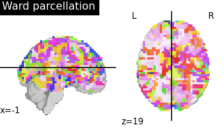
Using and visualizing the resulting parcellation#
Visualizing the parcellation#
The labels of the parcellation are found in the labels_img_ attribute of
the nilearn.regions.Parcellations object after fitting it to the data
using ward.fit. We directly use the result for visualization.
To visualize the clusters, we assign random colors to each cluster for the labels visualization.
Compressed representation#
The clustering can be used to transform the data into a smaller representation, taking the average on each parcel:
call ward.transform to obtain the mean value of each cluster (for each scan)
call ward.inverse_transform on the previous result to turn it back into the masked picture shape
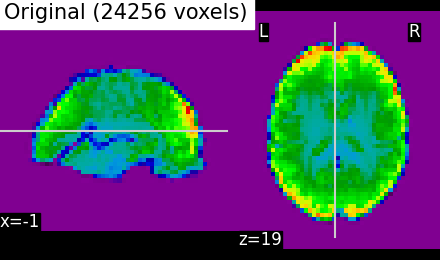
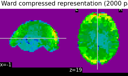
We can see that using only 2000 parcels, the original image is well approximated.
Example code
All the steps discussed in this section can be seen implemented in a full code example.