The haxby dataset: different multi-class strategies

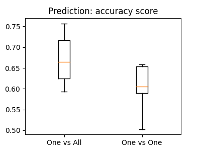
We compare one vs all and one vs one multi-class strategies: the overall cross-validated accuracy and the confusion matrix.

Note

If you are using Nilearn with a version older than 0.9.0, then you should either upgrade your version or import maskers from the input_data module instead of the maskers module.

That is, you should manually replace in the following example all occurrences of:

from nilearn.maskers import NiftiMasker

with:

from nilearn.input_data import NiftiMasker

Load the Haxby data dataset

from nilearn import datasets
import numpy as np
import pandas as pd
# By default 2nd subject from haxby datasets will be fetched.
haxby_dataset = datasets.fetch_haxby()

# Print basic information on the dataset
print('Mask nifti images are located at: %s' % haxby_dataset.mask)
print('Functional nifti images are located at: %s' % haxby_dataset.func[0])

func_filename = haxby_dataset.func[0]
mask_filename = haxby_dataset.mask

# Load the behavioral data that we will predict
labels = pd.read_csv(haxby_dataset.session_target[0], sep=" ")
y = labels['labels']
session = labels['chunks']

# Remove the rest condition, it is not very interesting
non_rest = (y != 'rest')
y = y[non_rest]

# Get the labels of the numerical conditions represented by the vector y
unique_conditions, order = np.unique(y, return_index=True)
# Sort the conditions by the order of appearance
unique_conditions = unique_conditions[np.argsort(order)]

Mask nifti images are located at: /home/alexis/nilearn_data/haxby2001/mask.nii.gz
Functional nifti images are located at: /home/alexis/nilearn_data/haxby2001/subj2/bold.nii.gz

Prepare the fMRI data

from nilearn.maskers import NiftiMasker
# For decoding, standardizing is often very important
nifti_masker = NiftiMasker(mask_img=mask_filename, standardize=True,
                           runs=session, smoothing_fwhm=4,
                           memory="nilearn_cache", memory_level=1)
X = nifti_masker.fit_transform(func_filename)

# Remove the "rest" condition
X = X[non_rest]
session = session[non_rest]

Build the decoders, using scikit-learn

Here we use a Support Vector Classification, with a linear kernel, and a simple feature selection step

from sklearn.svm import SVC
from sklearn.feature_selection import SelectKBest, f_classif
from sklearn.multiclass import OneVsOneClassifier, OneVsRestClassifier
from sklearn.pipeline import Pipeline

svc_ovo = OneVsOneClassifier(Pipeline([
    ('anova', SelectKBest(f_classif, k=500)),
    ('svc', SVC(kernel='linear'))
]))

svc_ova = OneVsRestClassifier(Pipeline([
    ('anova', SelectKBest(f_classif, k=500)),
    ('svc', SVC(kernel='linear'))
]))

Now we compute cross-validation scores

from sklearn.model_selection import cross_val_score

cv_scores_ovo = cross_val_score(svc_ovo, X, y, cv=5, verbose=1)

cv_scores_ova = cross_val_score(svc_ova, X, y, cv=5, verbose=1)

print('OvO:', cv_scores_ovo.mean())
print('OvA:', cv_scores_ova.mean())

[Parallel(n_jobs=1)]: Using backend SequentialBackend with 1 concurrent workers.
[Parallel(n_jobs=1)]: Done   5 out of   5 | elapsed:   12.1s finished
[Parallel(n_jobs=1)]: Using backend SequentialBackend with 1 concurrent workers.
[Parallel(n_jobs=1)]: Done   5 out of   5 | elapsed:    9.0s finished
OvO: 0.601855088049469
OvA: 0.6712058072321548

Plot barplots of the prediction scores

from matplotlib import pyplot as plt
plt.figure(figsize=(4, 3))
plt.boxplot([cv_scores_ova, cv_scores_ovo])
plt.xticks([1, 2], ['One vs All', 'One vs One'])
plt.title('Prediction: accuracy score')

Text(0.5, 1.0, 'Prediction: accuracy score')

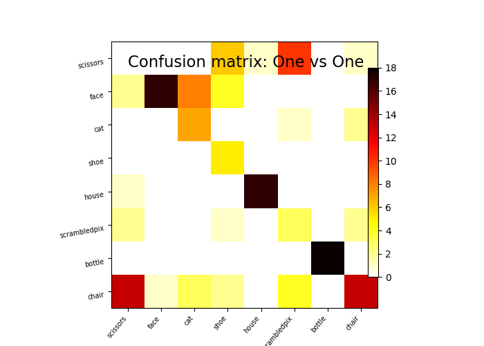
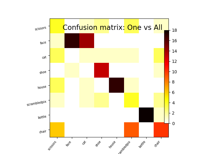
Plot a confusion matrix

We fit on the first 10 sessions and plot a confusion matrix on the last 2 sessions

from sklearn.metrics import confusion_matrix
from nilearn.plotting import plot_matrix, show

svc_ovo.fit(X[session < 10], y[session < 10])
y_pred_ovo = svc_ovo.predict(X[session >= 10])

plot_matrix(confusion_matrix(y_pred_ovo, y[session >= 10]),
            labels=unique_conditions,
            title='Confusion matrix: One vs One', cmap='hot_r')

svc_ova.fit(X[session < 10], y[session < 10])
y_pred_ova = svc_ova.predict(X[session >= 10])

plot_matrix(confusion_matrix(y_pred_ova, y[session >= 10]),
            labels=unique_conditions,
            title='Confusion matrix: One vs All', cmap='hot_r')

show()

• 
• 

Estimated memory usage: 2690 MB