Connectome extraction: inverse covariance for direct connections

Page summary

Given a set of time-series (eg as extracted in the previous section) A functional connectome is a set of connections representing brain interactions between regions. Here we show the use of sparse-inverse covariance to extract functional connectomes focussing only on direct interactions between regions.

References

• Smith et al, Network modelling methods for FMRI, NeuroImage 2011

• Varoquaux and Craddock, Learning and comparing functional connectomes across subjects, NeuroImage 2013

Sparse inverse covariance for functional connectomes

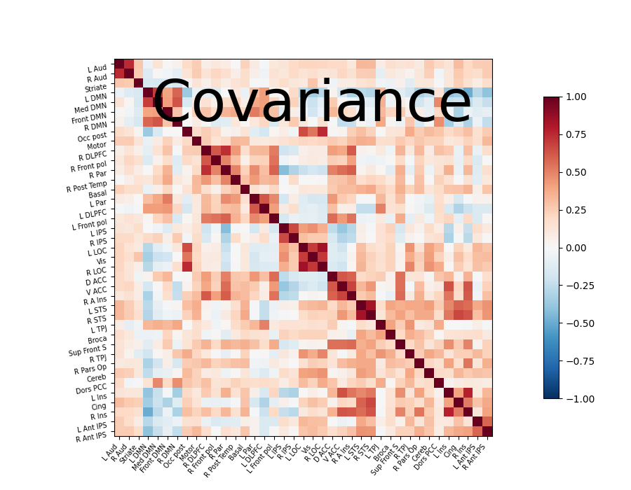
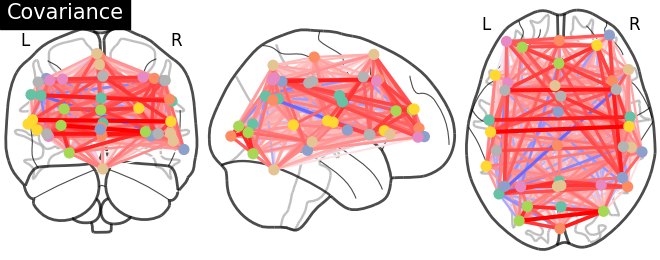
Functional connectivity can be obtained by estimating a covariance (or correlation) matrix for signals from different brain regions decomposed, for example on resting-state or naturalistic-stimuli datasets. The same information can be represented as a weighted graph, vertices being brain regions, weights on edges being covariances (gaussian graphical model). However, coefficients in a covariance matrix reflect direct as well as indirect connections. Covariance matrices form very dense brain connectomes, and it is rather difficult to extract from them only the direct connections between two regions.

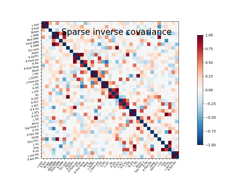
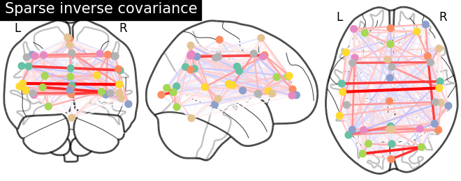
As shown in [Smith 2011], [Varoquaux 2010], it is more interesting to use the inverse covariance matrix, ie the precision matrix. It gives only direct connections between regions, as it contains partial covariances, which are covariances between two regions conditioned on all the others.

To recover well the interaction structure, a sparse inverse covariance estimator is necessary. The GraphicalLasso, implemented in scikit-learn’s estimator sklearn.covariance.GraphicalLassoCV is a good, simple solution. To use it, you need to create an estimator object:

>>> from sklearn.covariance import GraphicalLassoCV
>>> estimator = GraphicalLassoCV()

And then you can fit it on the activation time series, for instance extracted in the previous section:

>>> estimator.fit(time_series)  

The covariance matrix and inverse-covariance matrix (precision matrix) can be found respectively in the covariance_ and precision_ attribute of the estimator:

>>> estimator.covariance_  
>>> estimator.precision_  

Parameter selection

The parameter controlling the sparsity is set by cross-validation scheme. If you want to specify it manually, use the estimator sklearn.covariance.GraphicalLasso.

Full example

See the following example for a full file running the analysis: Computing a connectome with sparse inverse covariance

Exercise: computing sparse inverse covariance

Compute and visualize a connectome on the first subject of the brain development dataset downloaded with nilearn.datasets.fetch_development_fmri

Hints: The example above has the solution

Reference

• The graph lasso [Friedman et al, Biostatistics 2007] is useful to estimate one inverse covariance, ie to work on single-subject data or concatenate multi-subject data.

Sparse inverse covariance on multiple subjects

To work at the level of a group of subject, it can be interesting to estimate multiple connectomes for each, with a similar structure but differing connection values across subjects.

For this, nilearn provides the nilearn.connectome.GroupSparseCovarianceCV estimator. Its usage is similar to the GraphicalLassoCV object, but it takes a list of time series:

>>> estimator.fit([time_series_1, time_series_2, ...])  

And it provides one estimated covariance and inverse-covariance (precision) matrix per time-series: for the first one:

>>> estimator.covariances_[0]  
>>> estimator.precisions_[0]  

One specific case where this may be interesting is for group analysis across multiple subjects. Indeed, one challenge when doing statistics on the coefficients of a connectivity matrix is that the number of coefficients to compare grows quickly with the number of regions, and as a result correcting for multiple comparisons takes a heavy toll on statistical power.

In such a situation, you can use the GroupSparseCovariance and set an alpha value a bit higher than the alpha value selected by cross-validation in the GroupSparseCovarianceCV. Such a choice will enforce a stronger sparsity on the precision matrices for each subject. As the sparsity is common to each subject, you can then do the group analysis only on the non zero coefficients.

Full example

See the following example for a full file running the analysis: Group Sparse inverse covariance for multi-subject connectome

Exercise: computing the correlation matrix of rest fmri

Try using the information above to compute a connectome on the first 5 subjects of the brain development dataset downloaded with nilearn.datasets.fetch_development_fmri

Hint: The example above works through the solution for the ADHD dataset. adhd.

Reference

• The group-sparse covariance [Varoquaux et al, NIPS 2010]

Comparing the different approaches on simulated data

We simulate several sets of signals, one set representing one subject, with different precision matrices, but sharing a common sparsity pattern: 10 brain regions, for 20 subjects.

A single-subject estimation can be performed using the sklearn.covariance.GraphicalLassoCV estimator from scikit-learn.

It is also possible to fit a graph lasso on data from every subject all together.

Finally, we use the nilearn.connectome.GroupSparseCovarianceCV 1.

The results are the following:

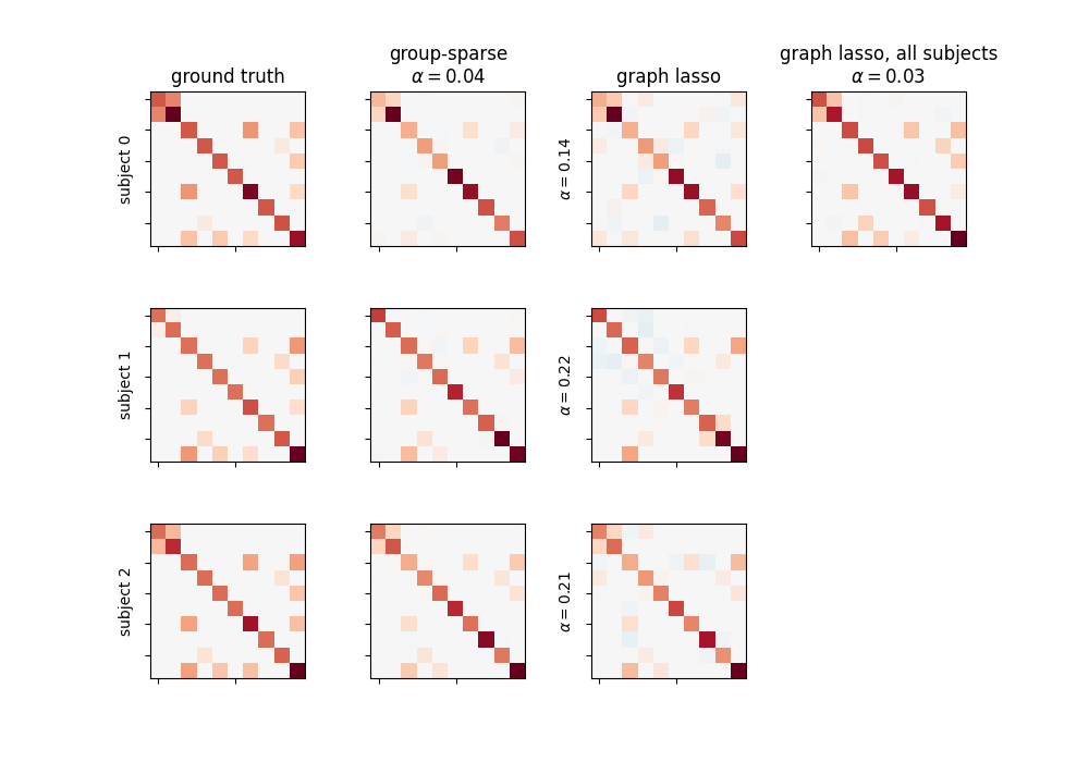
The group-sparse estimation outputs matrices with the same sparsity pattern, but different values for the non-zero coefficients. This is not the case for the graph lasso output, which all have similar but different structures. Note that the graph lasso applied to all subjects at once gives a sparsity pattern close to that obtained with the group-sparse one, but cannot provide per-subject information.

Full Example

The complete source code for this example can be found here: Connectivity structure estimation on simulated data

1

A lot of technical details on the algorithm used for group-sparse estimation and its implementation can be found in Group-sparse covariance estimation.

Reference

• The Brain covariance selection using population prior [Varoquaux et al, NIPS 2010]

Linking total and direct interactions at the group level

Individual connectivity patterns reflect both on covariances and inverse covariances, but in different ways. For multiple subjects, mean covariance (or correlation) and group sparse inverse covariance provide different insights into the connectivity at the group level.

We can go one step further by coupling the information from total (pairwise) and direct interactions in a unique group connectome. This can be done through a geometrical framework allowing to measure interactions in a common space called tangent space [Varoquaux et al, MICCAI 2010].

In nilearn, this is implemented in nilearn.connectome.ConnectivityMeasure:

>>> measure = ConnectivityMeasure(kind='tangent')  

The group connectivity is computed using all the subjects timeseries.:

>>> connectivities = measure.fit([time_series_1, time_series_2, ...])  
>>> group_connectivity = measure.mean_  

Deviations from this mean in the tangent space are provided in the connectivities array and can be used to compare different groups/sessions. In practice, the tangent measure can outperform the correlation and partial correlation measures, especially for noisy or heterogeneous data.

Full example

See the following example for a full file running the analysis: Classification of age groups using functional connectivity

Exercise: computing connectivity in tangent space

Compute and visualize the tangent group connectome based on the brain development dataset downloaded with nilearn.datasets.fetch_development_fmri

Hints: The example above has the solution

Reference

• The tangent space for connectivity [Varoquaux et al, MICCAI 2010]