Beta-Series Modeling for Task-Based Functional Connectivity and Decoding

This example shows how to run beta series GLM models, which are a common modeling approach for a variety of analyses of task-based fMRI data with an event-related task design, including functional connectivity, decoding, and representational similarity analysis.

Beta series models fit trial-wise conditions, which allow users to create “time series” of these trial-wise maps, which can be substituted for the typical time series used in resting-state functional connectivity analyses. Generally, these models are most useful for event-related task designs, while other modeling approaches, such as psychophysiological interactions (PPIs), tend to perform better in block designs, depending on the type of analysis. See Cisler et al.1 for more information about this, in the context of functional connectivity analyses.

Two of the most well-known beta series modeling methods are Least Squares- All (LSA) 2 and Least Squares- Separate (LSS) 34. In LSA, a single GLM is run, in which each trial of each condition of interest is separated out into its own condition within the design matrix. In LSS, each trial of each condition of interest has its own GLM, in which the targeted trial receives its own column within the design matrix, but everything else remains the same as the standard model. Trials are then looped across, and many GLMs are fitted, with the parameter estimate map extracted from each GLM to build the LSS beta series.

Choosing the right model for your analysis

We have chosen not to reproduce analyses systematically comparing beta series modeling approaches in nilearn’s documentation; however, we do incorporate recommendations from the literature. Rather than taking these recommendations at face value, please refer back to the original publications and any potential updates to the literature, when possible.

First, as mentioned above, according to Cisler et al.1, beta series models are most appropriate for event-related task designs. For block designs, a PPI model is better suited- at least for functional connectivity analyses.

According to Abdulrahman and Henson5, the decision between LSA and LSS should be based on three factors: inter-trial variability, scan noise, and stimulus onset timing. While Mumford et al.3 proposes LSS as a tool primarily for fast event-related designs (i.e., ones with short inter-trial intervals), Abdulrahman and Henson5 finds, in simulations, that LSA performs better than LSS when trial variability is greater than scan noise, even in fast designs.

Note

If you are using Nilearn with a version older than 0.9.0, then you should either upgrade your version or import maskers from the input_data module instead of the maskers module.

That is, you should manually replace in the following example all occurrences of:

from nilearn.maskers import NiftiMasker

with:

from nilearn.input_data import NiftiMasker

import matplotlib.pyplot as plt

from nilearn.glm.first_level import FirstLevelModel
from nilearn import image, plotting

Prepare data and analysis parameters

Download data in BIDS format and event information for one subject, and create a standard FirstLevelModel.

from nilearn.datasets import fetch_language_localizer_demo_dataset

data_dir, _ = fetch_language_localizer_demo_dataset()

from nilearn.glm.first_level import first_level_from_bids

models, models_run_imgs, events_dfs, models_confounds = \
    first_level_from_bids(
        data_dir,
        'languagelocalizer',
        img_filters=[('desc', 'preproc')],
    )

# Grab the first subject's model, functional file, and events DataFrame
standard_glm = models[0]
fmri_file = models_run_imgs[0][0]
events_df = events_dfs[0][0]

# We will use first_level_from_bids's parameters for the other models
glm_parameters = standard_glm.get_params()
# We need to override one parameter (signal_scaling) with the value of
# scaling_axis
glm_parameters['signal_scaling'] = standard_glm.scaling_axis

/home/alexis/miniconda3/envs/nilearn/lib/python3.10/site-packages/nilearn/glm/first_level/first_level.py:901: UserWarning:

SliceTimingRef not found in file /home/alexis/nilearn_data/fMRI-language-localizer-demo-dataset/derivatives/sub-01/func/sub-01_task-languagelocalizer_desc-preproc_bold.json. It will be assumed that the slice timing reference is 0.0 percent of the repetition time. If it is not the case it will need to be set manually in the generated list of models

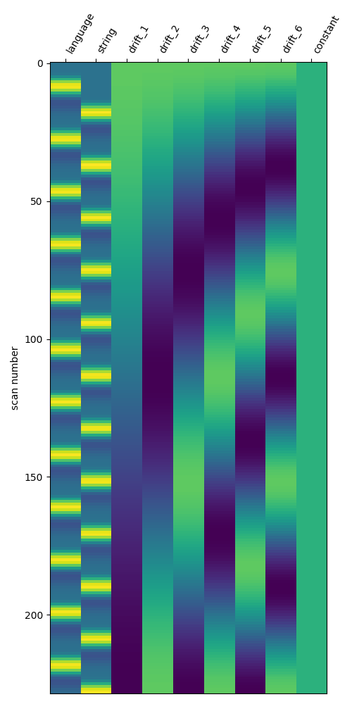
Define the standard model

Here, we create a basic GLM for this run, which we can use to highlight differences between the standard modeling approach and beta series models. We will just use the one created by first_level_from_bids.

standard_glm.fit(fmri_file, events_df)

# The standard design matrix has one column for each condition, along with
# columns for the confound regressors and drifts
fig, ax = plt.subplots(figsize=(5, 10))
plotting.plot_design_matrix(standard_glm.design_matrices_[0], ax=ax)
fig.show()

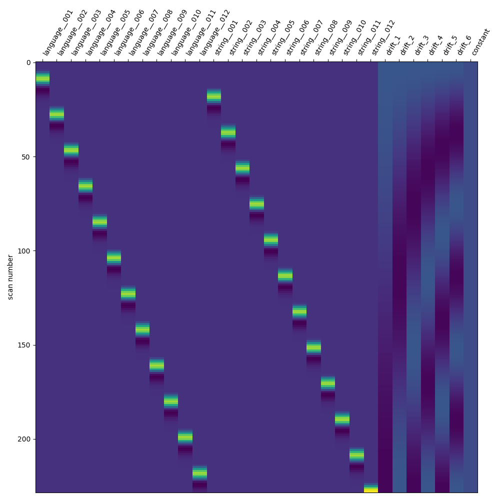
Define the LSA model

We will now create a least squares- all (LSA) model. This involves a simple transformation, where each trial of interest receives its own unique trial type. It’s important to ensure that the original trial types can be inferred from the updated trial-wise trial types, in order to collect the resulting beta maps into condition-wise beta series.

# Transform the DataFrame for LSA
lsa_events_df = events_df.copy()
conditions = lsa_events_df['trial_type'].unique()
condition_counter = {c: 0 for c in conditions}
for i_trial, trial in lsa_events_df.iterrows():
    trial_condition = trial['trial_type']
    condition_counter[trial_condition] += 1
    # We use a unique delimiter here (``__``) that shouldn't be in the
    # original condition names
    trial_name = f'{trial_condition}__{condition_counter[trial_condition]:03d}'
    lsa_events_df.loc[i_trial, 'trial_type'] = trial_name

lsa_glm = FirstLevelModel(**glm_parameters)
lsa_glm.fit(fmri_file, lsa_events_df)

fig, ax = plt.subplots(figsize=(10, 10))
plotting.plot_design_matrix(lsa_glm.design_matrices_[0], ax=ax)
fig.show()

Aggregate beta maps from the LSA model based on condition

Collect the parameter estimate maps

lsa_beta_maps = {cond: [] for cond in events_df['trial_type'].unique()}
trialwise_conditions = lsa_events_df['trial_type'].unique()
for condition in trialwise_conditions:
    beta_map = lsa_glm.compute_contrast(condition, output_type='effect_size')
    # Drop the trial number from the condition name to get the original name
    condition_name = condition.split('__')[0]
    lsa_beta_maps[condition_name].append(beta_map)

# We can concatenate the lists of 3D maps into a single 4D beta series for
# each condition, if we want
lsa_beta_maps = {
    name: image.concat_imgs(maps) for name, maps in lsa_beta_maps.items()
}

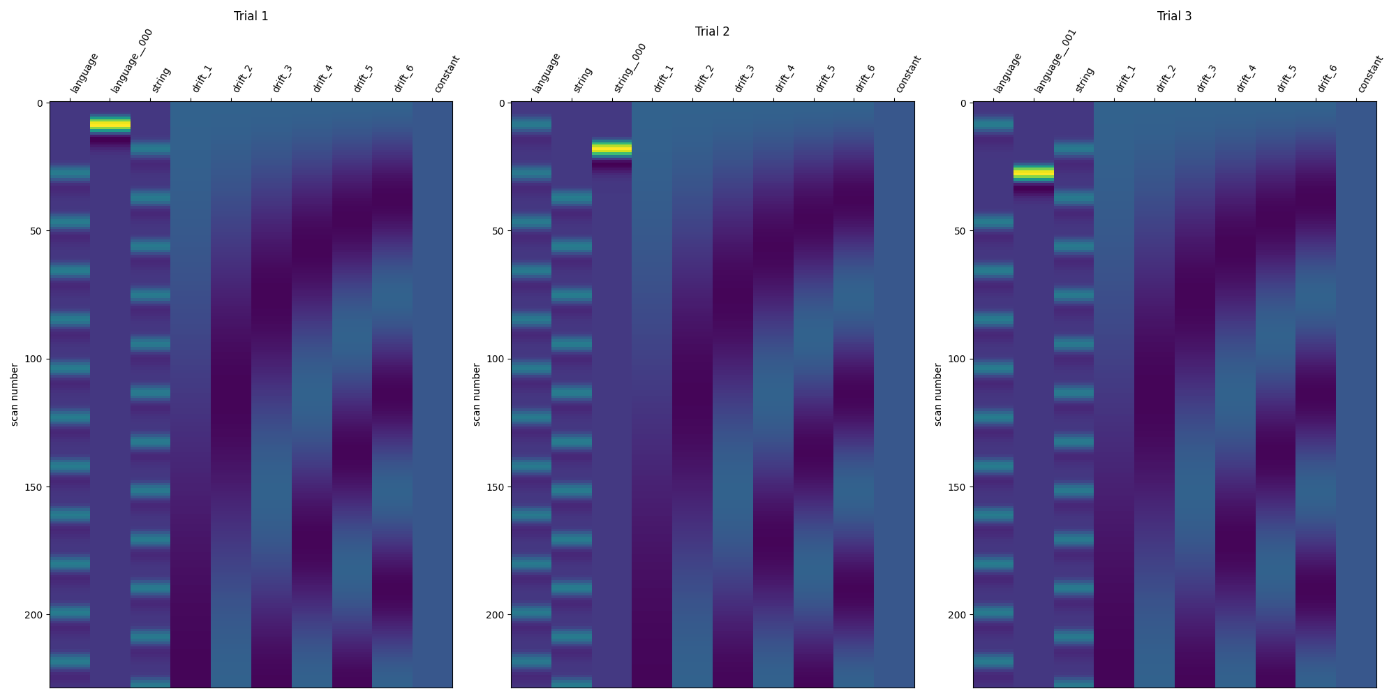
Define the LSS models

We will now create a separate LSS model for each trial of interest. The transformation is much like the LSA approach, except that we only relabel one trial in the DataFrame. We loop through the trials, create a version of the DataFrame where the targeted trial has a unique trial type, fit the model to that DataFrame, and finally collect the targeted trial’s beta map for the beta series.

def lss_transformer(df, row_number):
    """Label one trial for one LSS model.

    Parameters
    ----------
    df : pandas.DataFrame
        BIDS-compliant events file information.
    row_number : int
        Row number in the DataFrame.
        This indexes the trial that will be isolated.

    Returns
    -------
    df : pandas.DataFrame
        Update events information, with the select trial's trial type isolated.
    trial_name : str
        Name of the isolated trial's trial type.
    """
    df = df.copy()

    # Determine which number trial it is *within the condition*
    trial_condition = df.loc[row_number, 'trial_type']
    trial_type_series = df['trial_type']
    trial_type_series = trial_type_series.loc[
        trial_type_series == trial_condition
    ]
    trial_type_list = trial_type_series.index.tolist()
    trial_number = trial_type_list.index(row_number)

    # We use a unique delimiter here (``__``) that shouldn't be in the
    # original condition names.
    # Technically, all you need is for the requested trial to have a unique
    # 'trial_type' *within* the dataframe, rather than across models.
    # However, we may want to have meaningful 'trial_type's (e.g., 'Left_001')
    # across models, so that you could track individual trials across models.
    trial_name = f'{trial_condition}__{trial_number:03d}'
    df.loc[row_number, 'trial_type'] = trial_name
    return df, trial_name


# Loop through the trials of interest and transform the DataFrame for LSS
lss_beta_maps = {cond: [] for cond in events_df['trial_type'].unique()}
lss_design_matrices = []

for i_trial in range(events_df.shape[0]):
    lss_events_df, trial_condition = lss_transformer(events_df, i_trial)

    # Compute and collect beta maps
    lss_glm = FirstLevelModel(**glm_parameters)
    lss_glm.fit(fmri_file, lss_events_df)

    # We will save the design matrices across trials to show them later
    lss_design_matrices.append(lss_glm.design_matrices_[0])

    beta_map = lss_glm.compute_contrast(
        trial_condition,
        output_type='effect_size',
    )

    # Drop the trial number from the condition name to get the original name
    condition_name = trial_condition.split('__')[0]
    lss_beta_maps[condition_name].append(beta_map)

# We can concatenate the lists of 3D maps into a single 4D beta series for
# each condition, if we want
lss_beta_maps = {
    name: image.concat_imgs(maps) for name, maps in lss_beta_maps.items()
}

Show the design matrices for the first few trials

fig, axes = plt.subplots(ncols=3, figsize=(20, 10))
for i_trial in range(3):
    plotting.plot_design_matrix(
        lss_design_matrices[i_trial],
        ax=axes[i_trial],
    )
    axes[i_trial].set_title(f'Trial {i_trial + 1}')

fig.show()

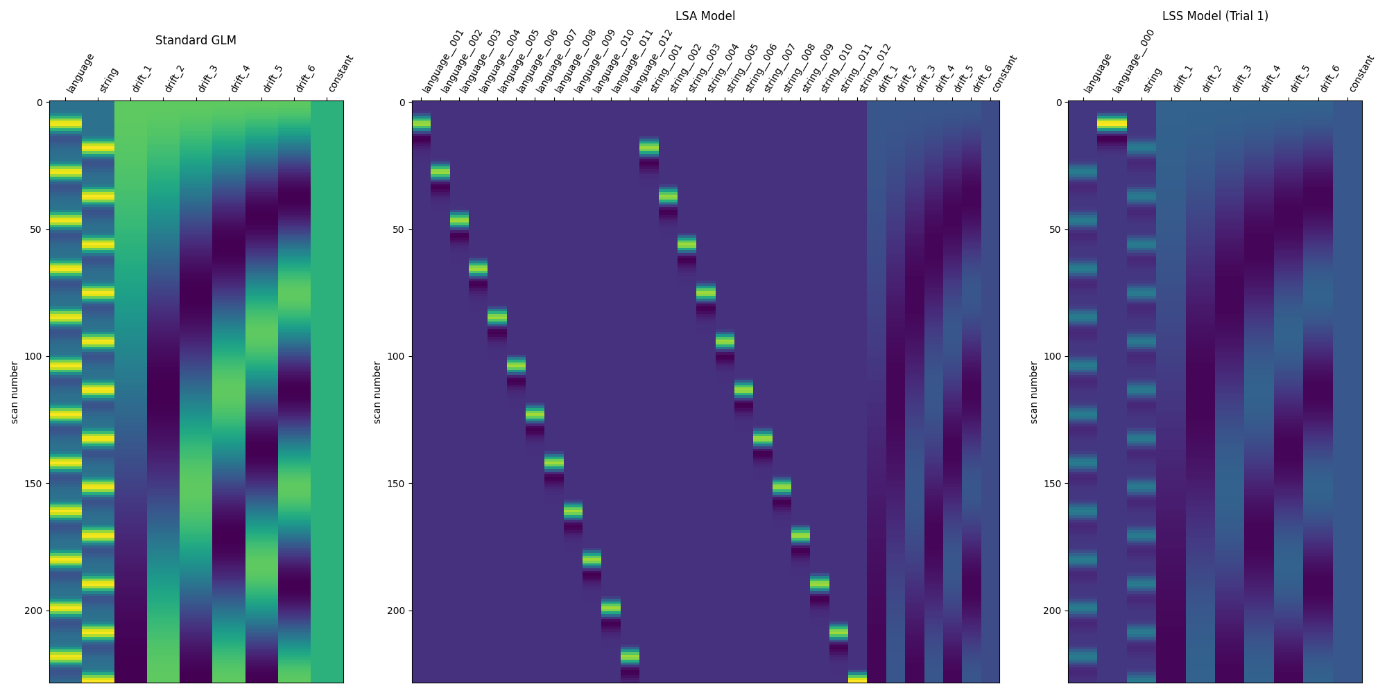
Compare the three modeling approaches

DM_TITLES = ['Standard GLM', 'LSA Model', 'LSS Model (Trial 1)']
DESIGN_MATRICES = [
    standard_glm.design_matrices_[0],
    lsa_glm.design_matrices_[0],
    lss_design_matrices[0],
]

fig, axes = plt.subplots(
    ncols=3,
    figsize=(20, 10),
    gridspec_kw={'width_ratios': [1, 2, 1]},
)

for i_ax, ax in enumerate(axes):
    plotting.plot_design_matrix(DESIGN_MATRICES[i_ax], ax=axes[i_ax])
    axes[i_ax].set_title(DM_TITLES[i_ax])

fig.show()

Applications of beta series

Beta series can be used much like resting-state data, though generally with vastly reduced degrees of freedom than a typical resting-state run, given that the number of trials should always be less than the number of volumes in a functional MRI run.

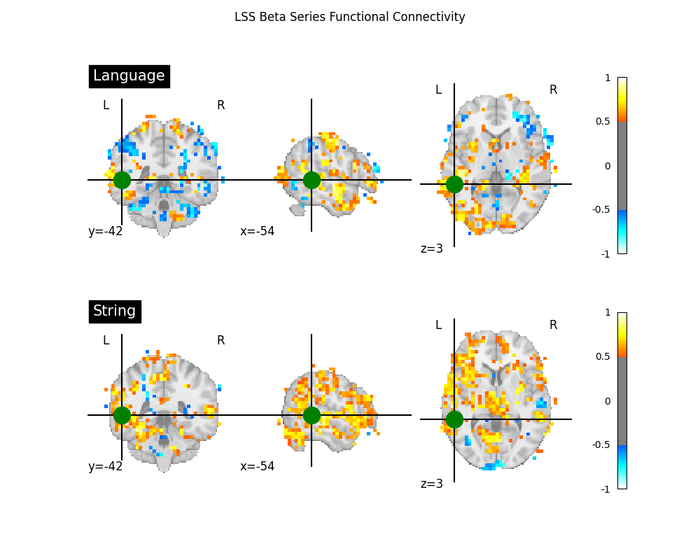
Two common applications of beta series are to functional connectivity and decoding analyses. For an example of a beta series applied to decoding, see Decoding of a dataset after GLM fit for signal extraction. Here, we show how the beta series can be applied to functional connectivity analysis. In the following section, we perform a quick task-based functional connectivity analysis of each of the two task conditions (‘language’ and ‘string’), using the LSS beta series. This section is based on Producing single subject maps of seed-to-voxel correlation, which goes into more detail about seed-to-voxel functional connectivity analyses.

import numpy as np

from nilearn.maskers import NiftiSpheresMasker, NiftiMasker

# Coordinate taken from Neurosynth's 'language' meta-analysis
coords = [(-54, -42, 3)]

# Initialize maskers for the seed and the rest of the brain
seed_masker = NiftiSpheresMasker(
    coords,
    radius=8,
    detrend=True,
    standardize=True,
    low_pass=None,
    high_pass=None,
    t_r=None,
    memory='nilearn_cache',
    memory_level=1,
    verbose=0,
)

brain_masker = NiftiMasker(
    smoothing_fwhm=6,
    detrend=True,
    standardize=True,
    low_pass=None,
    high_pass=None,
    t_r=None,
    memory='nilearn_cache',
    memory_level=1,
    verbose=0,
)

# Perform the seed-to-voxel correlation for the LSS 'language' beta series
lang_seed_beta_series = seed_masker.fit_transform(lss_beta_maps['language'])
lang_beta_series = brain_masker.fit_transform(lss_beta_maps['language'])
lang_corrs = np.dot(
    lang_beta_series.T,
    lang_seed_beta_series,
) / lang_seed_beta_series.shape[0]
language_connectivity_img = brain_masker.inverse_transform(lang_corrs.T)

# Perform the seed-to-voxel correlation for the LSS 'string' beta series
string_seed_beta_series = seed_masker.fit_transform(lss_beta_maps['string'])
string_beta_series = brain_masker.fit_transform(lss_beta_maps['string'])
string_corrs = np.dot(
    string_beta_series.T,
    string_seed_beta_series,
) / string_seed_beta_series.shape[0]
string_connectivity_img = brain_masker.inverse_transform(string_corrs.T)

# Show both correlation maps
fig, axes = plt.subplots(figsize=(10, 8), nrows=2)

display = plotting.plot_stat_map(
    language_connectivity_img,
    threshold=0.5,
    vmax=1,
    cut_coords=coords[0],
    title='Language',
    figure=fig,
    axes=axes[0],
)
display.add_markers(
    marker_coords=coords,
    marker_color='g',
    marker_size=300,
)

display = plotting.plot_stat_map(
    string_connectivity_img,
    threshold=0.5,
    vmax=1,
    cut_coords=coords[0],
    title='String',
    figure=fig,
    axes=axes[1],
)
display.add_markers(
    marker_coords=coords,
    marker_color='g',
    marker_size=300,
)
fig.suptitle('LSS Beta Series Functional Connectivity')

fig.show()

References

1(1,2)

Josh M Cisler, Keith Bush, and J Scott Steele. A comparison of statistical methods for detecting context-modulated functional connectivity in fmri. Neuroimage, 84:1042–1052, 2014.

2

Jesse Rissman, Adam Gazzaley, and Mark D’Esposito. Measuring functional connectivity during distinct stages of a cognitive task. Neuroimage, 23(2):752–763, 2004.

3(1,2)

Jeanette A Mumford, Benjamin O Turner, F Gregory Ashby, and Russell A Poldrack. Deconvolving bold activation in event-related designs for multivoxel pattern classification analyses. Neuroimage, 59(3):2636–2643, 2012.

4

Benjamin O Turner, Jeanette A Mumford, Russell A Poldrack, and F Gregory Ashby. Spatiotemporal activity estimation for multivoxel pattern analysis with rapid event-related designs. NeuroImage, 62(3):1429–1438, 2012.

5(1,2)

Hunar Abdulrahman and Richard N Henson. Effect of trial-to-trial variability on optimal event-related fmri design: implications for beta-series correlation and multi-voxel pattern analysis. NeuroImage, 125:756–766, 2016.

Estimated memory usage: 188 MB